In this activity, we classify the same objects as with Acitivity 18 and 19. The objects classified here in this activity are vcut and pillows. The output for vcut should be 0 and for pillow should be 1.
The code is written below:
N = [2,4,1];
train = fscanfMat("F:\AP 186\act20\training.txt")';// Training Set
train = train/max(train);
t = [0 0 0 0 1 1 1 1];
lp = [2.5,0];
W = ann_FF_init(N);
T = 1000; //Training cyles
W = ann_FF_Std_online(train,t,N,W,lp,T);
test = fscanfMat("F:\AP 186\act20\data4.txt")';
test = test/max(test);
class = ann_FF_run(test,N,W)
round(class)
The result of classification is 100% successful!
0.1069949 0.0069226 0.0023741 0.0146057 0.9982912 0.5178297 0.9649571 0.9974860
Rounding off values are given by:
0 0 0 0 1 1 1 1
In this activity, I will give myself a grade of 10/10 because of very good classification of the objects.
Sunday, October 12, 2008
Activity 19 - Probabilistic Classification
In this activity, two set of classes are used and their pattern are recognized via the Linear Discriminant Analysis (LDA). The classification rule is used to "assign an object to the group with highest conditional probability"[1]. The formula used to classify an object to its group is given by:

where µ is the mean corrected value of an object, C is the pooled covariance matrix of all the groups and p is the classification probability. Two sets of sample were used; Vcut chips (Figure 1)
and Pillows (Figure 2). The criterion used to classify the objects are their Mean of the red and the green values.
 Figure 1
 Figure 2
The results of the classification is given by Table 1.
 For the Training data, 100% classification was obtained as expected. But for the Test data, only 75% classification was obtained.
In conclusion, the LDA is a good method in classification of objects for random sample.
For this activity, I will give myself a grade of 8 because I did not obtain 100% classification for the test datas.
Appendix:
a = fscanfMat("F:\AP 186\act19\data1.txt");
b = fscanfMat("F:\AP 186\act19\data2.txt");
q = fscanfMat("F:\AP 186\act19\data4.txt");
c(1:4,1:2) = a(1:4,1:2);
c(5:8,1:2) = b(1:4,1:2);
mean_g = mean(c,'r');
a1(1:4,1:2) = a(1:4,1:2);
b1(1:4,1:2) = b(1:4,1:2);
mean_a1 = mean(a1,'r');
mean_b1 = mean(b1,'r');
for i = 1:2
mean_cora1(:,i) = a(:,i)-mean_g(i);
mean_corb1(:,i) = b(:,i)-mean_g(i);
end
c1 = (mean_cora1'*mean_cora1)/4;
c2 = (mean_corb1'*mean_corb1)/4;
for i = 1:2
for j = 1:2
C(i,j) = (4/8)*c1(i,j)+(4/8)*c2(i,j);
end
end
f(:,1) = ((((mean_a1)*inv(C))*c' )-(0.5*((mean_a1*inv(C))*mean_a1'))+log(0.5))';
f(:,2) = ((((mean_b1)*inv(C))*c' )-(0.5*((mean_b1*inv(C))*mean_b1'))+log(0.5))';
Saturday, October 4, 2008
Activity 18 - Pattern Recognition
In this activity, we gathered different samples with same quantities. Our samples are Piatos, Pillows, Kwek-Kwek and Vcut. Per sample, we gathered 8 of this samples.
Half of these samples are the training samples and half are the test samples. To identify the membership of the test samples to what classification it belongs, feature of that sample and the training samples should be obtained. For example, the color of the training samples of piatos should share the same color as the test samples of piatos.
The mean of the feature vectors are extracted from the training samples. In my case, the feature vectors I used are the mean and the standard deviation of the red and grenn values of the training samples. I added all features vectors and values are given below:
piatos = 0.8979285
vcut = 0.9626847
kwek-kwek = 1.0137804
pillows = 0.9057169
Same feature vectors were also obtained from the test samples and obtaied the sum of these feature vectors. To find the classification of that test sample, the summed feature vector of the test sample is subtracted to the summed feature vector of the training sample and find where it is minimum. The results are given below:
Note that for samples Pillow and Piatos, the percentage of classification did not obtain a perfect classification becuase the feature vector has small difference. But for both Vcut and KwekKwek, 100% classification were obtained.
For this activity, I will give myself a grade of 8 because I think I've met all the objectives though the classification was'nt perfect.
Appendix:
Source code:
I = [];
I1 = [];
for i =5:8
for i =5:8
I = imread("kwekkwek" + string(i) + ".JPG");
I1 = imread("kwekkwekc"+string(i)+".JPG");
r1 = I(:,:,1)./(I(:,:,1)+I(:,:,2)+I(:,:,3));
g1 = I(:,:,2)./(I(:,:,1)+I(:,:,2)+I(:,:,3));
b1 = I(:,:,3)./(I(:,:,1)+I(:,:,2)+I(:,:,3));
r2 = I1(:,:,1)./(I1(:,:,1)+I1(:,:,2)+I1(:,:,3));
g2 = I1(:,:,2)./(I1(:,:,1)+I1(:,:,2)+I1(:,:,3));
b2 = I1(:,:,3)./(I1(:,:,1)+I1(:,:,2)+I1(:,:,3));
r2_1 = floor(r2*255); g2_1 = floor(g2*255);
Standr2(i) = stdev(r2);
Standg2(i) = stdev(g2);
Meanr2(i) = mean(r2);
Meang2(i) = mean(g2);
pr = (1/(stdev(r2)*sqrt(2*%pi)))*exp(-1*((r1-mean(r2)).^2/(2*stdev(r2)))); pg = (1/(stdev(g2)*sqrt(2*%pi)))*exp(-1*((g1-mean(g2)).^2/(2*stdev(g2))));
new = (pr.*pg);
new2 = new/max(new);
new3 = im2bw(new2,0.7);
[x,y] = follow(new3);
n = size(x);
x2 = x;
y2 = y;
x2(1) = x(n(1));
x2(2:n(1))=x(1:(n(1)-1));
y2(1) = y(n(1));
y2(2:n(1))=y(1:(n(1)-1));
area(i) = abs(0.5*sum(x.*y2 - y.*x2));//Green's Theorem imwrite(new3,"pill" + string(i)+".JPG");
end
training = [0.8979285 0.9626847 1.0137804 0.9057169];
training = [0.8979285 0.9626847 1.0137804 0.9057169];
train = mean(Meanr2(1:4))+mean(Meang2(1:4))+mean(Standr2(1:4))+mean(Standg2(1:4));
for i = 1:4
for j = 1:4
test(i,j) = abs((Meanr2(4+i) +Meang2(4+i) + Standr2(4+i) + Standg2(4+i)) - training(j));
end
end
Monday, September 29, 2008
Activity 17 - Video Processing
In this activity, video processing was done. First, the video is ripped to create images representing frames in the video. The images obtained were then processed.
The video used in this activity is a rolling object on an inclined plane. The objective of this activity is to obtain the acceleration seen from the video and compare it to theoretical values given some parameters.
The images obtained from the video were converted to binary images. The centroid of the rolling cylinder for all the images were obtained and plot the distance from the origin versus the frame. The plot is given below:

Conversion of values from pixel to millimeter and frame to time were performed through known values in the video (for example, the size of the rolling cylinder and the frame rate). Curve fitting was then performed to the plot to obtain a polynomial equation of distance that depends on the constant acceleration and velocity which is given by:
d = 331.69 t^2 + 21.002 t^2
from the equation, the acceleration is given by 331.69x2 = 663.38 mm/sec^2 (which is the acceleration along the x - axis since the video was viewed from the top).
Theoretical calculation of the acceleration given by the equations below revealed that for that same parameter, the acceleration is 592.71 mm/sec^2. Large difference from theoretical and experimental values maybe due to the centroid finding of the object.

For this activity, I would give myself a grade of 8. I would like to acknowledge the help of Abraham Latimer Camba for the theoretical computation of the acceleration.
Appendix:
//15 frames per second
I = [];
se = [1 1;1 1];
for i =1:15
I = imread("vid" + string(i) + ".jpeg");
I1 = im2bw(I,0.7);
I2 = erode(dilate(I1,se),se);
I3 = erode(I2,se);
imwrite(I3,"videos" + string(i)+".jpeg");
[x1,y1] = find(I3==1);
x(i)=mean(x1);
y(i)=mean(y1);
end
distancey = y - min(y);
distancex = x - min(x);
distance = sqrt(distancex^2 + distancey^2);
for i = 1:15
velocity(1) = distancey(1);
velocity(i+1) = distance(i+1) - distancey(i);
end
for i = 1:15
acceleration(1) = 0;
acceleration(i+1) = velocity(i+1) - velocity(i);
end
scf(0);plot(distance);
scf(1);plot(velocity);
scf(2);plot(acceleration);
The video used in this activity is a rolling object on an inclined plane. The objective of this activity is to obtain the acceleration seen from the video and compare it to theoretical values given some parameters.
(I cannot upload the video because of large file size)..
The images obtained from the video were converted to binary images. The centroid of the rolling cylinder for all the images were obtained and plot the distance from the origin versus the frame. The plot is given below:

Conversion of values from pixel to millimeter and frame to time were performed through known values in the video (for example, the size of the rolling cylinder and the frame rate). Curve fitting was then performed to the plot to obtain a polynomial equation of distance that depends on the constant acceleration and velocity which is given by:
d = 331.69 t^2 + 21.002 t^2
from the equation, the acceleration is given by 331.69x2 = 663.38 mm/sec^2 (which is the acceleration along the x - axis since the video was viewed from the top).
Theoretical calculation of the acceleration given by the equations below revealed that for that same parameter, the acceleration is 592.71 mm/sec^2. Large difference from theoretical and experimental values maybe due to the centroid finding of the object.

For this activity, I would give myself a grade of 8. I would like to acknowledge the help of Abraham Latimer Camba for the theoretical computation of the acceleration.
Appendix:
//15 frames per second
I = [];
se = [1 1;1 1];
for i =1:15
I = imread("vid" + string(i) + ".jpeg");
I1 = im2bw(I,0.7);
I2 = erode(dilate(I1,se),se);
I3 = erode(I2,se);
imwrite(I3,"videos" + string(i)+".jpeg");
[x1,y1] = find(I3==1);
x(i)=mean(x1);
y(i)=mean(y1);
end
distancey = y - min(y);
distancex = x - min(x);
distance = sqrt(distancex^2 + distancey^2);
for i = 1:15
velocity(1) = distancey(1);
velocity(i+1) = distance(i+1) - distancey(i);
end
for i = 1:15
acceleration(1) = 0;
acceleration(i+1) = velocity(i+1) - velocity(i);
end
scf(0);plot(distance);
scf(1);plot(velocity);
scf(2);plot(acceleration);
Wednesday, September 17, 2008
Activity 16 - Color Image Segmentation
In this activity, a sample from the whole image is picked out to get the Region Of Interest (ROI) from the image.
Example of this is the human skin recognition.
There are two basic techniques in segmentation; (1) Probability Distribution Estimation and (2) Histogram Backprojection.
The image and the used in this activity is shown below:
Figure 1. The original image
 Figure 2. Sample from the original image
Probability Distribution Estimation
In this technique, a sample from the original image is cropped from the original image. Per pixel, the r value and the g of both the original image and the cropped image are normalized by dividing it to the sum of r, g and b values of that pixel. The probability that the the r value and the g value of the original image belong to the ROI is given by the equation:
 Equation 1

Example of this is the human skin recognition.
There are two basic techniques in segmentation; (1) Probability Distribution Estimation and (2) Histogram Backprojection.
The image and the used in this activity is shown below:

Figure 1. The original image
 Figure 2. Sample from the original image
Probability Distribution Estimation
In this technique, a sample from the original image is cropped from the original image. Per pixel, the r value and the g of both the original image and the cropped image are normalized by dividing it to the sum of r, g and b values of that pixel. The probability that the the r value and the g value of the original image belong to the ROI is given by the equation:
 Equation 1
The resulting ROI is shown below: Figure 3
 Figure 3
Histogram Backprojection
In this technique, the 2D histogram of the portion of the original image was obtained. The obtained histogram was normalized to obtain the probability distribution function(PDF). The r and the g values of the original image per pixel were back-projected (or replaced) by finding the r and the g values from the PDF. The resulting image is shown below:
In this technique, the 2D histogram of the portion of the original image was obtained. The obtained histogram was normalized to obtain the probability distribution function(PDF). The r and the g values of the original image per pixel were back-projected (or replaced) by finding the r and the g values from the PDF. The resulting image is shown below:

Figure 4
Comparing the two techniques, for me the Probability Distribution Estimation is a better technique for segmentation because of the expected ROI was obtained. In contrast to the Histogram Back-projection, not all the expected ROI was obtained.
For this activity, I will give ,myself a grade of 8 because of the late submission.
I would like to acknowledge Abraham Latimer Camba for helping me in the Histogram Back-projection part.
Appendix:
Source code
//First: Segmentation via probability
I = imread("F:\AP 186\act16\pic.jpg");
I2 = imread("F:\AP 186\act16\small.jpg");
n1 = size(I);
scf(1);imshow(I);
r1 = I(:,:,1)./(I(:,:,1)+I(:,:,2)+I(:,:,3));
g1 = I(:,:,2)./(I(:,:,1)+I(:,:,2)+I(:,:,3));
b1 = I(:,:,3)./(I(:,:,1)+I(:,:,2)+I(:,:,3));
r2 = I2(:,:,1)./(I2(:,:,1)+I2(:,:,2)+I2(:,:,3));
g2 = I2(:,:,2)./(I2(:,:,1)+I2(:,:,2)+I2(:,:,3));
b2 = I2(:,:,3)./(I2(:,:,1)+I2(:,:,2)+I2(:,:,3));
pr = (1/(stdev(r2)*sqrt(2*%pi)))*exp(-1*((r1-mean(r2)).^2/(2*stdev(r2))));
pg = (1/(stdev(g2)*sqrt(2*%pi)))*exp(-1*((g1-mean(g2)).^2/(2*stdev(g2))));
new = (pr.*pg);
scf(3);imshow((new),[]);
//Second: Segmentation via Histogram
r2_1 = floor(r2*255);
g2_1 = floor(g2*255);
n = size(r2);
Hist = zeros(256,256);
for i = 1:n(1)
for j =1:n(2)
x = r2_1(i,j)+1;
y = g2_1(i,j)+1;
Hist(x,y) = Hist(x,y) +1;
end
end
scf(5);plot3d(0:255,0:255,Hist);
Hist = Hist/max(Hist);
scf(2);imshow(log(Hist+0.0000000001),[]);
r1 = round(r1*255);
g1 = round(g1*255);
for i = 1:n1(1)
for j = 1:n1(2)
T(i,j) = Hist(r1(i,j)+1,g1(i,j)+1);
end
end
scf(4);imshow(T,[]);
imwrite(new/max(new),"F:\AP 186\act16\1_1.jpg");
imwrite(T,"F:\AP 186\act16\2_2.jpg");
Activity 15 - Color Image Processing
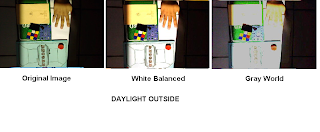
In this activity, images having unbalanced colored images were enhanced by;
(1) White Balancing,
(2) Gray World Balancing
White Balancing:
White balancing technique uses a known white object from the image for balancing. The red, green and blue of the RGB values of the known white object in the image is used as "NORMALIZING" or as divider for all the RGB values of all the pixels in the image.
Gray World Balancing:
Gray balancing technique uses the mean of all the red, green and blue values present in the image as the divider for all the RGB values of the pixels present in the image.
Here are some examples of images that were white balanced and gray balanced:


 For this activity, I will give myself a grade of 7 out of 10 because of the late submission.
I would like to acknowledge Mark Leo for helping me debug errors on my program.
Appendix:
Source code for White Balancing created in Scilab:
I = imread("C:\Documents and Settings\AP186user15\Desktop\act15\outside - daylight.jpg");
imshow(I);
n = size(I);
RGB = round(locate(1,flag=1));
r = I((RGB(1)),(RGB(2)),1);
g = I((RGB(1)),(RGB(2)),2);
b = I((RGB(1)),(RGB(2)),3);
Ibal(:,:,1) = I(:,:,1)/r;
Ibal(:,:,2) = I(:,:,2)/g;
Ibal(:,:,3) = I(:,:,3)/b;
index=find(Ibal>1.0);
Ibal(index)=1.0;
//Inew(:,:,1) = Ibal(:,:,1)/max(I(:,:,1));
//Inew(:,:,2) = Ibal(:,:,2)/max(I(:,:,2));
//Inew(:,:,3) = Ibal(:,:,3)/max(I(:,:,3));
imwrite(Ibal,"C:\Documents and Settings\AP186user15\Desktop\act15\outside - daylight_bal.jpg");
Source code for Gray World Balancing:
I = imread("C:\Documents and Settings\AP186user15\Desktop\act15\o- incandescent.jpg");
//imshow(I);
//n = size(I);
//RGB = round(locate(1,flag=1));
r = mean(I(:,:,1));
g = mean(I(:,:,2));
b = mean(I(:,:,3));
Ibal(:,:,1) = I(:,:,1)/r;
Ibal(:,:,2) = I(:,:,2)/g;
Ibal(:,:,3) = I(:,:,3)/b;
index=find(Ibal>1.0);
Ibal(index)=1.0;
Ibal = 0.75*Ibal;
//Inew(:,:,1) = Ibal(:,:,1)/max(I(:,:,1));
//Inew(:,:,2) = Ibal(:,:,2)/max(I(:,:,2));
//Inew(:,:,3) = Ibal(:,:,3)/max(I(:,:,3));
imwrite(Ibal,"C:\Documents and Settings\AP186user15\Desktop\act15\o- incandescent_bal_gray.jpg");
Subscribe to:
Posts (Atom)