In this activity, we classify the same objects as with Acitivity 18 and 19. The objects classified here in this activity are vcut and pillows. The output for vcut should be 0 and for pillow should be 1.
The code is written below:
N = [2,4,1];
train = fscanfMat("F:\AP 186\act20\training.txt")';// Training Set
train = train/max(train);
t = [0 0 0 0 1 1 1 1];
lp = [2.5,0];
W = ann_FF_init(N);
T = 1000; //Training cyles
W = ann_FF_Std_online(train,t,N,W,lp,T);
test = fscanfMat("F:\AP 186\act20\data4.txt")';
test = test/max(test);
class = ann_FF_run(test,N,W)
round(class)
The result of classification is 100% successful!
0.1069949 0.0069226 0.0023741 0.0146057 0.9982912 0.5178297 0.9649571 0.9974860
Rounding off values are given by:
0 0 0 0 1 1 1 1
In this activity, I will give myself a grade of 10/10 because of very good classification of the objects.
Sunday, October 12, 2008
Activity 19 - Probabilistic Classification
In this activity, two set of classes are used and their pattern are recognized via the Linear Discriminant Analysis (LDA). The classification rule is used to "assign an object to the group with highest conditional probability"[1]. The formula used to classify an object to its group is given by:

where µ is the mean corrected value of an object, C is the pooled covariance matrix of all the groups and p is the classification probability. Two sets of sample were used; Vcut chips (Figure 1)
and Pillows (Figure 2). The criterion used to classify the objects are their Mean of the red and the green values.
 Figure 1
 Figure 2
The results of the classification is given by Table 1.
 For the Training data, 100% classification was obtained as expected. But for the Test data, only 75% classification was obtained.
In conclusion, the LDA is a good method in classification of objects for random sample.
For this activity, I will give myself a grade of 8 because I did not obtain 100% classification for the test datas.
Appendix:
a = fscanfMat("F:\AP 186\act19\data1.txt");
b = fscanfMat("F:\AP 186\act19\data2.txt");
q = fscanfMat("F:\AP 186\act19\data4.txt");
c(1:4,1:2) = a(1:4,1:2);
c(5:8,1:2) = b(1:4,1:2);
mean_g = mean(c,'r');
a1(1:4,1:2) = a(1:4,1:2);
b1(1:4,1:2) = b(1:4,1:2);
mean_a1 = mean(a1,'r');
mean_b1 = mean(b1,'r');
for i = 1:2
mean_cora1(:,i) = a(:,i)-mean_g(i);
mean_corb1(:,i) = b(:,i)-mean_g(i);
end
c1 = (mean_cora1'*mean_cora1)/4;
c2 = (mean_corb1'*mean_corb1)/4;
for i = 1:2
for j = 1:2
C(i,j) = (4/8)*c1(i,j)+(4/8)*c2(i,j);
end
end
f(:,1) = ((((mean_a1)*inv(C))*c' )-(0.5*((mean_a1*inv(C))*mean_a1'))+log(0.5))';
f(:,2) = ((((mean_b1)*inv(C))*c' )-(0.5*((mean_b1*inv(C))*mean_b1'))+log(0.5))';
Saturday, October 4, 2008
Activity 18 - Pattern Recognition
In this activity, we gathered different samples with same quantities. Our samples are Piatos, Pillows, Kwek-Kwek and Vcut. Per sample, we gathered 8 of this samples.
Half of these samples are the training samples and half are the test samples. To identify the membership of the test samples to what classification it belongs, feature of that sample and the training samples should be obtained. For example, the color of the training samples of piatos should share the same color as the test samples of piatos.
The mean of the feature vectors are extracted from the training samples. In my case, the feature vectors I used are the mean and the standard deviation of the red and grenn values of the training samples. I added all features vectors and values are given below:
piatos = 0.8979285
vcut = 0.9626847
kwek-kwek = 1.0137804
pillows = 0.9057169
Same feature vectors were also obtained from the test samples and obtaied the sum of these feature vectors. To find the classification of that test sample, the summed feature vector of the test sample is subtracted to the summed feature vector of the training sample and find where it is minimum. The results are given below:
Note that for samples Pillow and Piatos, the percentage of classification did not obtain a perfect classification becuase the feature vector has small difference. But for both Vcut and KwekKwek, 100% classification were obtained.
For this activity, I will give myself a grade of 8 because I think I've met all the objectives though the classification was'nt perfect.
Appendix:
Source code:
I = [];
I1 = [];
for i =5:8
for i =5:8
I = imread("kwekkwek" + string(i) + ".JPG");
I1 = imread("kwekkwekc"+string(i)+".JPG");
r1 = I(:,:,1)./(I(:,:,1)+I(:,:,2)+I(:,:,3));
g1 = I(:,:,2)./(I(:,:,1)+I(:,:,2)+I(:,:,3));
b1 = I(:,:,3)./(I(:,:,1)+I(:,:,2)+I(:,:,3));
r2 = I1(:,:,1)./(I1(:,:,1)+I1(:,:,2)+I1(:,:,3));
g2 = I1(:,:,2)./(I1(:,:,1)+I1(:,:,2)+I1(:,:,3));
b2 = I1(:,:,3)./(I1(:,:,1)+I1(:,:,2)+I1(:,:,3));
r2_1 = floor(r2*255); g2_1 = floor(g2*255);
Standr2(i) = stdev(r2);
Standg2(i) = stdev(g2);
Meanr2(i) = mean(r2);
Meang2(i) = mean(g2);
pr = (1/(stdev(r2)*sqrt(2*%pi)))*exp(-1*((r1-mean(r2)).^2/(2*stdev(r2)))); pg = (1/(stdev(g2)*sqrt(2*%pi)))*exp(-1*((g1-mean(g2)).^2/(2*stdev(g2))));
new = (pr.*pg);
new2 = new/max(new);
new3 = im2bw(new2,0.7);
[x,y] = follow(new3);
n = size(x);
x2 = x;
y2 = y;
x2(1) = x(n(1));
x2(2:n(1))=x(1:(n(1)-1));
y2(1) = y(n(1));
y2(2:n(1))=y(1:(n(1)-1));
area(i) = abs(0.5*sum(x.*y2 - y.*x2));//Green's Theorem imwrite(new3,"pill" + string(i)+".JPG");
end
training = [0.8979285 0.9626847 1.0137804 0.9057169];
training = [0.8979285 0.9626847 1.0137804 0.9057169];
train = mean(Meanr2(1:4))+mean(Meang2(1:4))+mean(Standr2(1:4))+mean(Standg2(1:4));
for i = 1:4
for j = 1:4
test(i,j) = abs((Meanr2(4+i) +Meang2(4+i) + Standr2(4+i) + Standg2(4+i)) - training(j));
end
end
Monday, September 29, 2008
Activity 17 - Video Processing
In this activity, video processing was done. First, the video is ripped to create images representing frames in the video. The images obtained were then processed.
The video used in this activity is a rolling object on an inclined plane. The objective of this activity is to obtain the acceleration seen from the video and compare it to theoretical values given some parameters.
The images obtained from the video were converted to binary images. The centroid of the rolling cylinder for all the images were obtained and plot the distance from the origin versus the frame. The plot is given below:

Conversion of values from pixel to millimeter and frame to time were performed through known values in the video (for example, the size of the rolling cylinder and the frame rate). Curve fitting was then performed to the plot to obtain a polynomial equation of distance that depends on the constant acceleration and velocity which is given by:
d = 331.69 t^2 + 21.002 t^2
from the equation, the acceleration is given by 331.69x2 = 663.38 mm/sec^2 (which is the acceleration along the x - axis since the video was viewed from the top).
Theoretical calculation of the acceleration given by the equations below revealed that for that same parameter, the acceleration is 592.71 mm/sec^2. Large difference from theoretical and experimental values maybe due to the centroid finding of the object.

For this activity, I would give myself a grade of 8. I would like to acknowledge the help of Abraham Latimer Camba for the theoretical computation of the acceleration.
Appendix:
//15 frames per second
I = [];
se = [1 1;1 1];
for i =1:15
I = imread("vid" + string(i) + ".jpeg");
I1 = im2bw(I,0.7);
I2 = erode(dilate(I1,se),se);
I3 = erode(I2,se);
imwrite(I3,"videos" + string(i)+".jpeg");
[x1,y1] = find(I3==1);
x(i)=mean(x1);
y(i)=mean(y1);
end
distancey = y - min(y);
distancex = x - min(x);
distance = sqrt(distancex^2 + distancey^2);
for i = 1:15
velocity(1) = distancey(1);
velocity(i+1) = distance(i+1) - distancey(i);
end
for i = 1:15
acceleration(1) = 0;
acceleration(i+1) = velocity(i+1) - velocity(i);
end
scf(0);plot(distance);
scf(1);plot(velocity);
scf(2);plot(acceleration);
The video used in this activity is a rolling object on an inclined plane. The objective of this activity is to obtain the acceleration seen from the video and compare it to theoretical values given some parameters.
(I cannot upload the video because of large file size)..
The images obtained from the video were converted to binary images. The centroid of the rolling cylinder for all the images were obtained and plot the distance from the origin versus the frame. The plot is given below:

Conversion of values from pixel to millimeter and frame to time were performed through known values in the video (for example, the size of the rolling cylinder and the frame rate). Curve fitting was then performed to the plot to obtain a polynomial equation of distance that depends on the constant acceleration and velocity which is given by:
d = 331.69 t^2 + 21.002 t^2
from the equation, the acceleration is given by 331.69x2 = 663.38 mm/sec^2 (which is the acceleration along the x - axis since the video was viewed from the top).
Theoretical calculation of the acceleration given by the equations below revealed that for that same parameter, the acceleration is 592.71 mm/sec^2. Large difference from theoretical and experimental values maybe due to the centroid finding of the object.

For this activity, I would give myself a grade of 8. I would like to acknowledge the help of Abraham Latimer Camba for the theoretical computation of the acceleration.
Appendix:
//15 frames per second
I = [];
se = [1 1;1 1];
for i =1:15
I = imread("vid" + string(i) + ".jpeg");
I1 = im2bw(I,0.7);
I2 = erode(dilate(I1,se),se);
I3 = erode(I2,se);
imwrite(I3,"videos" + string(i)+".jpeg");
[x1,y1] = find(I3==1);
x(i)=mean(x1);
y(i)=mean(y1);
end
distancey = y - min(y);
distancex = x - min(x);
distance = sqrt(distancex^2 + distancey^2);
for i = 1:15
velocity(1) = distancey(1);
velocity(i+1) = distance(i+1) - distancey(i);
end
for i = 1:15
acceleration(1) = 0;
acceleration(i+1) = velocity(i+1) - velocity(i);
end
scf(0);plot(distance);
scf(1);plot(velocity);
scf(2);plot(acceleration);
Wednesday, September 17, 2008
Activity 16 - Color Image Segmentation
In this activity, a sample from the whole image is picked out to get the Region Of Interest (ROI) from the image.
Example of this is the human skin recognition.
There are two basic techniques in segmentation; (1) Probability Distribution Estimation and (2) Histogram Backprojection.
The image and the used in this activity is shown below:
Figure 1. The original image
 Figure 2. Sample from the original image
Probability Distribution Estimation
In this technique, a sample from the original image is cropped from the original image. Per pixel, the r value and the g of both the original image and the cropped image are normalized by dividing it to the sum of r, g and b values of that pixel. The probability that the the r value and the g value of the original image belong to the ROI is given by the equation:
 Equation 1

Example of this is the human skin recognition.
There are two basic techniques in segmentation; (1) Probability Distribution Estimation and (2) Histogram Backprojection.
The image and the used in this activity is shown below:

Figure 1. The original image
 Figure 2. Sample from the original image
Probability Distribution Estimation
In this technique, a sample from the original image is cropped from the original image. Per pixel, the r value and the g of both the original image and the cropped image are normalized by dividing it to the sum of r, g and b values of that pixel. The probability that the the r value and the g value of the original image belong to the ROI is given by the equation:
 Equation 1
The resulting ROI is shown below: Figure 3
 Figure 3
Histogram Backprojection
In this technique, the 2D histogram of the portion of the original image was obtained. The obtained histogram was normalized to obtain the probability distribution function(PDF). The r and the g values of the original image per pixel were back-projected (or replaced) by finding the r and the g values from the PDF. The resulting image is shown below:
In this technique, the 2D histogram of the portion of the original image was obtained. The obtained histogram was normalized to obtain the probability distribution function(PDF). The r and the g values of the original image per pixel were back-projected (or replaced) by finding the r and the g values from the PDF. The resulting image is shown below:

Figure 4
Comparing the two techniques, for me the Probability Distribution Estimation is a better technique for segmentation because of the expected ROI was obtained. In contrast to the Histogram Back-projection, not all the expected ROI was obtained.
For this activity, I will give ,myself a grade of 8 because of the late submission.
I would like to acknowledge Abraham Latimer Camba for helping me in the Histogram Back-projection part.
Appendix:
Source code
//First: Segmentation via probability
I = imread("F:\AP 186\act16\pic.jpg");
I2 = imread("F:\AP 186\act16\small.jpg");
n1 = size(I);
scf(1);imshow(I);
r1 = I(:,:,1)./(I(:,:,1)+I(:,:,2)+I(:,:,3));
g1 = I(:,:,2)./(I(:,:,1)+I(:,:,2)+I(:,:,3));
b1 = I(:,:,3)./(I(:,:,1)+I(:,:,2)+I(:,:,3));
r2 = I2(:,:,1)./(I2(:,:,1)+I2(:,:,2)+I2(:,:,3));
g2 = I2(:,:,2)./(I2(:,:,1)+I2(:,:,2)+I2(:,:,3));
b2 = I2(:,:,3)./(I2(:,:,1)+I2(:,:,2)+I2(:,:,3));
pr = (1/(stdev(r2)*sqrt(2*%pi)))*exp(-1*((r1-mean(r2)).^2/(2*stdev(r2))));
pg = (1/(stdev(g2)*sqrt(2*%pi)))*exp(-1*((g1-mean(g2)).^2/(2*stdev(g2))));
new = (pr.*pg);
scf(3);imshow((new),[]);
//Second: Segmentation via Histogram
r2_1 = floor(r2*255);
g2_1 = floor(g2*255);
n = size(r2);
Hist = zeros(256,256);
for i = 1:n(1)
for j =1:n(2)
x = r2_1(i,j)+1;
y = g2_1(i,j)+1;
Hist(x,y) = Hist(x,y) +1;
end
end
scf(5);plot3d(0:255,0:255,Hist);
Hist = Hist/max(Hist);
scf(2);imshow(log(Hist+0.0000000001),[]);
r1 = round(r1*255);
g1 = round(g1*255);
for i = 1:n1(1)
for j = 1:n1(2)
T(i,j) = Hist(r1(i,j)+1,g1(i,j)+1);
end
end
scf(4);imshow(T,[]);
imwrite(new/max(new),"F:\AP 186\act16\1_1.jpg");
imwrite(T,"F:\AP 186\act16\2_2.jpg");
Activity 15 - Color Image Processing
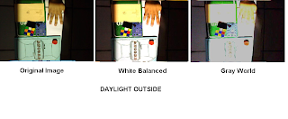
In this activity, images having unbalanced colored images were enhanced by;
(1) White Balancing,
(2) Gray World Balancing
White Balancing:
White balancing technique uses a known white object from the image for balancing. The red, green and blue of the RGB values of the known white object in the image is used as "NORMALIZING" or as divider for all the RGB values of all the pixels in the image.
Gray World Balancing:
Gray balancing technique uses the mean of all the red, green and blue values present in the image as the divider for all the RGB values of the pixels present in the image.
Here are some examples of images that were white balanced and gray balanced:


 For this activity, I will give myself a grade of 7 out of 10 because of the late submission.
I would like to acknowledge Mark Leo for helping me debug errors on my program.
Appendix:
Source code for White Balancing created in Scilab:
I = imread("C:\Documents and Settings\AP186user15\Desktop\act15\outside - daylight.jpg");
imshow(I);
n = size(I);
RGB = round(locate(1,flag=1));
r = I((RGB(1)),(RGB(2)),1);
g = I((RGB(1)),(RGB(2)),2);
b = I((RGB(1)),(RGB(2)),3);
Ibal(:,:,1) = I(:,:,1)/r;
Ibal(:,:,2) = I(:,:,2)/g;
Ibal(:,:,3) = I(:,:,3)/b;
index=find(Ibal>1.0);
Ibal(index)=1.0;
//Inew(:,:,1) = Ibal(:,:,1)/max(I(:,:,1));
//Inew(:,:,2) = Ibal(:,:,2)/max(I(:,:,2));
//Inew(:,:,3) = Ibal(:,:,3)/max(I(:,:,3));
imwrite(Ibal,"C:\Documents and Settings\AP186user15\Desktop\act15\outside - daylight_bal.jpg");
Source code for Gray World Balancing:
I = imread("C:\Documents and Settings\AP186user15\Desktop\act15\o- incandescent.jpg");
//imshow(I);
//n = size(I);
//RGB = round(locate(1,flag=1));
r = mean(I(:,:,1));
g = mean(I(:,:,2));
b = mean(I(:,:,3));
Ibal(:,:,1) = I(:,:,1)/r;
Ibal(:,:,2) = I(:,:,2)/g;
Ibal(:,:,3) = I(:,:,3)/b;
index=find(Ibal>1.0);
Ibal(index)=1.0;
Ibal = 0.75*Ibal;
//Inew(:,:,1) = Ibal(:,:,1)/max(I(:,:,1));
//Inew(:,:,2) = Ibal(:,:,2)/max(I(:,:,2));
//Inew(:,:,3) = Ibal(:,:,3)/max(I(:,:,3));
imwrite(Ibal,"C:\Documents and Settings\AP186user15\Desktop\act15\o- incandescent_bal_gray.jpg");
Wednesday, August 6, 2008
A13 – Photometric Stereo
In this activity, an object illuminated by same point source with 4 different location in reference to the object. The resulting images have different shadings. The objective of this activity is to predict the original shape of the image.
Letting the matrix V be the three dimensional position of the point source for different positions given and matrix I be the resulting image depending on the position of the light source. For each image with size (NxN), the images are then reshaped to (N^2 x 1) to form a column matrix. All of the reshaped images are then combined to form a single matrix I.
Matrix g contains all the information about the original shape about object and can be solved using Equation 1:
 Equation 1
Getting then normal vector of the g matrix, I used the Equation 2:
 Equation 2
 Equation 2
To know the shape of the object, we get the function f first by partial differentiation of normal vectors (x and y) with respect to z using Equation 3: Equation 3
 Equation 3
Finally, function f can be obtained using Equation 4:
 Equation 4
The result of the shape of the image is shown below:

 Equation 4
Figure 1
For this activity, I will give myself a grade of 10 because all of the objectives of the activity were met.
Appendix (Source code in Scilab):
loadmatfile ('C:\Documents and Settings\AP186user15\Desktop\ap18657activity13\Photos.mat');
browsevar();
I(1,:) = (I1(:))';
I(2,:) = (I2(:))';
I(3,:) = (I3(:))';
I(4,:) = (I4(:))';
V(1,:) = [0.085832 0.17365 0.98106];
V(2,:) = [0.085832 -0.17365 0.98106];
V(3,:) = [0.17365 0 0.98481];
V(4,:) = [0.16318 -0.34202 0.92542];
g = (inv(V'*V)*(V'))*I;
N = size(g);
gmag = [];
for i = 1:N(2)
gmag(i) = sqrt(g(1,i)**2 + g(2,i)**2 + g(3,i)**3)+0.0000000001;
end
n(1,:) = g(1,:)./gmag(1,:);
n(2,:) = g(2,:)./gmag(1,:);
n(3,:) = g(3,:)./gmag(1,:)+0.0000000001;
Fx = -n(1,:)./n(3,:);
Fy = -n(2,:)./n(3,:);
f = cumsum(Fx,1)+cumsum(Fy,2);
newf = matrix(f,[128,128]);
plot3d(1:128,1:128,newf)
Wednesday, July 30, 2008
Activity 11 - Camera Calibration
In this activity, we captured an image of a checker board with 1 inch by 1 inch dimension of each square. These 3D object is then transform it into a 2D image by the camera. The objective of this activity is to compute the Transformation Matrix present into the camera that transforms from world to camera coordinates given by the simple equation:

where G is the transformation matrix, xi and yi are the image coordinates and xw, yw and zw are the world coordinates.
25 differents spots on the image (xi's and yi's) and the corresponding world coordinates of the spots (xw, yw and zw) were taken. Plugging in it into the equation given by:
 Equation 2
Note: xo, yo and zo are the same as the xw, yw and zw.
 Figure 1 . Image used in calibration
The column matrix with components a is the transformation matrix.The values of a can easily be calculated by the equation: Equation 3
where Q matrix is the leftmost matrix in Equation 2 and d matrix is the rightmost matrix in Equation 2.
The values of the transformation matrix are:
- 11.158755
16.994741
- 0.3046630
81.972117
- 4.4211357
- 3.0139446
- 19.251234
271.84956
- 0.0126526
- 0.0067189
0.0023006
To verify if the transformation matrix is correct, 12 different spots(which were not used in the calibration) from the image were then taken and predicted the location of the spots using the transformation matrix given by the equation:

The results of the predicted location with comparison with the actual location using locate function in scilab is shown below:

In this activity, I will give myself a grade of 10 because the % errors I got are considerably low. I also acknowledge Abraham Latimer Camba for lending me the picture I used in this activity and Rafael Jaculbia for teaching how to use the locate function in scilab.
Appendix:
Source code in scilab
Image_mat1 = imread("F:\AP 186\activity 11\new.jpg");
gray = im2gray(Image_mat1);
imshow(gray);
Image_mat = locate(25,flag=1)';
Object_mat = fscanfMat("F:\AP 186\activity 11\Object.txt");
No = size(Object_mat);
Ni = size(Image_mat);
No2 = No(1)*2;
O = [];
for i = 1:No2
if modulo(i,2) == 1
k = ((i+1)/2);
O(i,1) = Object_mat((i+1)/2,1);
O(i,2) = Object_mat((i+1)/2,2);
O(i,3) = Object_mat((i+1)/2,3);
O(i,4) = 1;
O(i,5:8) = 0;
O(i,9) = -1*(Object_mat(k,1)*Image_mat(k,1));
O(i,10) = -1*(Object_mat(k,2)*Image_mat(k,1));
O(i,11) = -1*(Object_mat(k,3)*Image_mat(k,1));
end
if modulo(i,2)==0
O(i,5) = Object_mat(i*0.5,1);
O(i,6) = Object_mat(i*0.5,2);
O(i,7) = Object_mat(i*0.5,3);
O(i,8) = 1;
O(i,1:4) = 0;
O(i,9) = -1*(Object_mat(i*0.5,1)*Image_mat((i+1)/2,2));
O(i,10) = -1*(Object_mat(i*0.5,2)*Image_mat((i+1)/2,2));
O(i,11) = -1*(Object_mat(i*0.5,3)*Image_mat((i+1)/2,2));
end
end
d = [];
for i = 1:No2
if modulo(i,2)==1
d(i) = Image_mat(((i+1)/2),1);
end
if modulo(i,2) == 0
d(i) = Image_mat(i/2,2);
end
end
a = (inv(O'*O)*O')*d;
New_o = fscanfMat("F:\AP 186\activity 11\Object2.txt");
w = size(New_o);
y = [];
z = [];
for i = 1:w(1)
y(i) = (a(1,1)*New_o(i,1) +a(2,1)*New_o(i,2)+a(3,1)*New_o(i,3)+a(4,1))/(a(9,1)*New_o(i,1) +a(10,1)*New_o(i,2)+a(11,1)*New_o(i,3)+1);
z(i) = (a(5,1)*New_o(i,1) +a(6,1)*New_o(i,2)+a(7,1)*New_o(i,3)+a(8,1))/(a(9,1)*New_o(i,1) +a(10,1)*New_o(i,2)+a(11,1)*New_o(i,3)+1);
end
imshow(gray);
f = locate(12,flag=1);
Source:
[1] Activity manual and lectures provided by Dr. Maricor Soriano on her Applied Physics 186 class

Equation 1
where G is the transformation matrix, xi and yi are the image coordinates and xw, yw and zw are the world coordinates.
25 differents spots on the image (xi's and yi's) and the corresponding world coordinates of the spots (xw, yw and zw) were taken. Plugging in it into the equation given by:
 Equation 2
 Figure 1 . Image used in calibration
Note: The white dots are the points used for the calibration process and the red cross marks are the points that were predicted
 Equation 3
where Q matrix is the leftmost matrix in Equation 2 and d matrix is the rightmost matrix in Equation 2.
The values of the transformation matrix are:
- 11.158755
16.994741
- 0.3046630
81.972117
- 4.4211357
- 3.0139446
- 19.251234
271.84956
- 0.0126526
- 0.0067189
0.0023006
To verify if the transformation matrix is correct, 12 different spots(which were not used in the calibration) from the image were then taken and predicted the location of the spots using the transformation matrix given by the equation:

Equation 4
Note: a34 is set to 1.The results of the predicted location with comparison with the actual location using locate function in scilab is shown below:

In this activity, I will give myself a grade of 10 because the % errors I got are considerably low. I also acknowledge Abraham Latimer Camba for lending me the picture I used in this activity and Rafael Jaculbia for teaching how to use the locate function in scilab.
Appendix:
Source code in scilab
Image_mat1 = imread("F:\AP 186\activity 11\new.jpg");
gray = im2gray(Image_mat1);
imshow(gray);
Image_mat = locate(25,flag=1)';
Object_mat = fscanfMat("F:\AP 186\activity 11\Object.txt");
No = size(Object_mat);
Ni = size(Image_mat);
No2 = No(1)*2;
O = [];
for i = 1:No2
if modulo(i,2) == 1
k = ((i+1)/2);
O(i,1) = Object_mat((i+1)/2,1);
O(i,2) = Object_mat((i+1)/2,2);
O(i,3) = Object_mat((i+1)/2,3);
O(i,4) = 1;
O(i,5:8) = 0;
O(i,9) = -1*(Object_mat(k,1)*Image_mat(k,1));
O(i,10) = -1*(Object_mat(k,2)*Image_mat(k,1));
O(i,11) = -1*(Object_mat(k,3)*Image_mat(k,1));
end
if modulo(i,2)==0
O(i,5) = Object_mat(i*0.5,1);
O(i,6) = Object_mat(i*0.5,2);
O(i,7) = Object_mat(i*0.5,3);
O(i,8) = 1;
O(i,1:4) = 0;
O(i,9) = -1*(Object_mat(i*0.5,1)*Image_mat((i+1)/2,2));
O(i,10) = -1*(Object_mat(i*0.5,2)*Image_mat((i+1)/2,2));
O(i,11) = -1*(Object_mat(i*0.5,3)*Image_mat((i+1)/2,2));
end
end
d = [];
for i = 1:No2
if modulo(i,2)==1
d(i) = Image_mat(((i+1)/2),1);
end
if modulo(i,2) == 0
d(i) = Image_mat(i/2,2);
end
end
a = (inv(O'*O)*O')*d;
New_o = fscanfMat("F:\AP 186\activity 11\Object2.txt");
w = size(New_o);
y = [];
z = [];
for i = 1:w(1)
y(i) = (a(1,1)*New_o(i,1) +a(2,1)*New_o(i,2)+a(3,1)*New_o(i,3)+a(4,1))/(a(9,1)*New_o(i,1) +a(10,1)*New_o(i,2)+a(11,1)*New_o(i,3)+1);
z(i) = (a(5,1)*New_o(i,1) +a(6,1)*New_o(i,2)+a(7,1)*New_o(i,3)+a(8,1))/(a(9,1)*New_o(i,1) +a(10,1)*New_o(i,2)+a(11,1)*New_o(i,3)+1);
end
imshow(gray);
f = locate(12,flag=1);
Source:
[1] Activity manual and lectures provided by Dr. Maricor Soriano on her Applied Physics 186 class
Tuesday, July 22, 2008
A10 – Preprocessing Handwritten Text
In this activity, we are to remove an image cropped from a larger image which have horizontal lines by filtering. The original image is shown in Figure 1.
 Figure 1. Original Image
After filtering the image in its Fourier Space, I binarized the image and did some closing morphological operation using a 2x2 square image as the structuring element. Finally, I labelled the image and used the hotcolormap function in scilab to separate the labelled parts of the image.
I will give myself a grade of 9 because some of the horizontal lines were not removed.
Appendix:
Source Code in Scilab:
a= imread("G:\AP 186\Activity 10\image.jpg");
b = im2gray(a);
g = imread("G:\AP 186\Activity 10\filter3.bmp");
h = im2gray(g);
filter1 = fftshift(h);
c= (fft2(b));
scf(1);imshow(b,[]);
d = (fft2(filter1.*c));
I = abs(fft2(fft2(d)));
scf(2);imshow(I,[]);
w = I/max(I);
q = floor(255*w);
mat = size(q);
newpict = q;
for i = 1:mat(1) // Number of rows
for j = 1:mat(2) // Number of columns
if newpict(i,j) <>
newpict(i,j) = 0;
else
newpict(i,j) = 1;
end
end
end
SE_sq = [];
for i = 1:2
for j =1:2
SE_sq(i,j) = 1;
end
end
//
//SE_cross(1:3,1:3)=0;
//SE_cross(2,1:3) = 1;
//SE_cross(1:3,2) = 1;
//////////////////////////
p = abs(newpict-1);
Image_close1 = erode(dilate(p,SE_sq),SE_sq);//Closing
//Image_open1 = dilate(erode(Image_close1,SE_cross),SE_cross);//Opening
Invert = abs(Image_close1 - 1);
scf(3);imshow(Invert,[]);
o = bwlabel(Image_close1);
scf(4); imshow(o,[]);xset("colormap",hotcolormap(255));
scf(5); imshow(Invert,[]);
 Figure 1. Original Image
After filtering the image in its Fourier Space, I binarized the image and did some closing morphological operation using a 2x2 square image as the structuring element. Finally, I labelled the image and used the hotcolormap function in scilab to separate the labelled parts of the image.

Figure 2. Result
I will give myself a grade of 9 because some of the horizontal lines were not removed.
Appendix:
Source Code in Scilab:
a= imread("G:\AP 186\Activity 10\image.jpg");
b = im2gray(a);
g = imread("G:\AP 186\Activity 10\filter3.bmp");
h = im2gray(g);
filter1 = fftshift(h);
c= (fft2(b));
scf(1);imshow(b,[]);
d = (fft2(filter1.*c));
I = abs(fft2(fft2(d)));
scf(2);imshow(I,[]);
w = I/max(I);
q = floor(255*w);
mat = size(q);
newpict = q;
for i = 1:mat(1) // Number of rows
for j = 1:mat(2) // Number of columns
if newpict(i,j) <>
newpict(i,j) = 0;
else
newpict(i,j) = 1;
end
end
end
SE_sq = [];
for i = 1:2
for j =1:2
SE_sq(i,j) = 1;
end
end
//
//SE_cross(1:3,1:3)=0;
//SE_cross(2,1:3) = 1;
//SE_cross(1:3,2) = 1;
//////////////////////////
p = abs(newpict-1);
Image_close1 = erode(dilate(p,SE_sq),SE_sq);//Closing
//Image_open1 = dilate(erode(Image_close1,SE_cross),SE_cross);//Opening
Invert = abs(Image_close1 - 1);
scf(3);imshow(Invert,[]);
o = bwlabel(Image_close1);
scf(4); imshow(o,[]);xset("colormap",hotcolormap(255));
scf(5); imshow(Invert,[]);
Activity 9: Binary Operations
In image-based measurements, it is often desired that the region of interest (ROI) is made well segmented from the background either by edge detection (defining contours) or by specifying the ROI as a blob. Raw images must generally be preprocessed to make them suitable for further analysis.
Binarizing an image simplifies the separation of background from ROI. However, the optimum threshold must be found by examing the histogram.
In this activity, paper cut outs (with equal areas) were scanned in a flat bed scanner. The image was cropped in different positions and saved in a different image file. Each cropped image file was then processed by separating it from the background and binarizing the image file. After the binarization process the image file, morphological operations were done to eliminate pixels which were not to be the region of interest the ; the closing operation and the opening operation, which are just combinations of erosion and dilation operation. The structuring element used in the program was a 4x4 square image. The original image file is shown in Figure 1.

Figure 1. Original scanned image of cut outs
Problem encountered in approximating the area was the overlapping of circles which cannot be separated by my program. These overlaps gave me large area which obviously I can simply eliminate in my data. I limit my data on areas from 400 pixels to 600 pixels because greater or less than this range were considered to be noise or overlapping. Histogram of the areas is shown on Figure 2. Figure 2. Histogram of approximate area
 Figure 2. Histogram of approximate area
 The mean of the histogram is 541.4821 pixels and the standard deviation is 17.3184.
In this activity, I acknowledge the help of Rafael Jaculbia on how to get the histogram of my data in Microsoft Office Excel 2007. I will give myself a grade of 10 because I believe that I did all my best in this activity.
Appendix:
Source code in Scilab:
pict = imread("E:\AP 186\Act9\cropped11.jpg");
pict2 = im2gray(pict);
mat = size(pict);
newpict = pict2;
for i = 1:mat(1) // Number of rows
for j = 1:mat(2) // Number of columns
if newpict(i,j) < se_sq =" [];" i =" 1:4" j ="1:4" image_close1 =" erode(dilate(newpict,SE_sq),SE_sq);//Closing" image_open1 =" dilate(erode(Image_close1,SE_sq),SE_sq);//Opening" image_close2 =" erode(dilate(Image_open1,SE_sq),SE_sq);//Closing" image_open2 =" dilate(erode(Image_close2,SE_sq),SE_sq);//Opening" labelled =" bwlabel(Image_open2);//" count =" []" i =" 1:max(Labelled)" w =" find(Labelled" k =" size(w);">
Source:
[1] Activity 9 manual provided by Dr. Maricor Soriano
Tuesday, July 15, 2008
Activity 8: Morphological Operations
Mathematical morphology is a set-theoretical approach to multi-dimensional digital signal or image analysis, based on shape. The signals are locally compared with so-called structuring elements S of arbitrary shape with a reference point R.
The eroded image of an object O with respect to a structuring element S with a reference point R, ![]() , is the set of all reference points for which S is completely contained in O.
, is the set of all reference points for which S is completely contained in O.
The dilated image of an object O with respect to a structuring element S with a reference point R, ![]() , is the set of all reference points for which O and S have at least one common point.
, is the set of all reference points for which O and S have at least one common point.
Here are some examples of images that are eroded and dilated:


I would like to acknowledge Rafael Jaculbia for lending me his image templates I used in getting the erosion and dilation. I also acknowledge Billy Narag and Abraham Latimer Camba for helping understand idea of dilation and erosion.
For this activity, I would give myself a grade of 9 for the reason that I am not sure of some of my results because I did not correspond on my guess image.
Reference:
http://ikpe1101.ikp.kfa-juelich.de/briefbook_data_analysis/node178.html
Thursday, July 10, 2008
Enhancement in the Frequency Dom
Part 1:(FFT of 2D sine function)
Increasing the frequency of the 2D sine function increases the separation of the peak frequency in the FFT space and by rotating the sine function by some angle also rotates the peak frequency in the FFT space.
Multiplication of two sine function create a four peaks in the FFT space. The spacing of the peaks depends on the frequency of the of each sine. If the two sine functions have different frequencies, the peaks will not form a perfect square.


Part 2: (Finger Print)
Source code for finger print improvement:
a = imread("E:\AP 186\activity 7\finger ko.bmp");//image read
b = im2gray(a);
IM=fft(b,-1);
h1=mkfftfilter(b,'butterworth1',5);
h2=mkfftfilter(b,'butterworth2',30);
h=(h1-h2)*255;//Create filter
c = fft2(b);
apergrayshift = fftshift(h);
FR = apergrayshift.*(c);
IRA = (fft2(FR));
scf(1)
imshow(abs(fft2(fft2(IRA))),[]);
scf(2)
imshow(b,[]);
Part 3: (Space image improvement)
There is a given a image having vertical lines with uniform spacing, we can eliminate these vertical lines by taking the 2D Fourier Transform. By creating a filter which blocks the cross line on the Fourier Space of the original image, we can eliminate the vertical line present on the image. The FFT, the filter and the resulting image is shown below:


Collaborators:
Rafael Jaculbia, Elizabeth Anne Prieto
In this activity,I will give myself myself a grade of 7 because I believe that I did not obtain the right result for the second part.
Monday, July 7, 2008
Fourier Transform Model of Image
Part A: Fourier Transform of an Image
The Fourier Transform (FT) is one among the many classes of linear transforms that recast information into another set of linear basis. In particular, FT converts a signal with dimension X into a signal with dimension 1/X. If the signal has dimensions of space, a Fourier Transform of the signal will be inverse space or spatial frequency. The FT of an image f(x,y) is given by:
F ( f x , f y )=∫∫ f ( x , y) exp(−i 2pi( f x x f y y )) dx dy
This part of the activity discusses mainly on getting the fourier transform of the image and returning to its original image (meaning getting the fourier transform twice) . Getting the fourier transform twice will give an inverted original image. The simple source code is written below (at the appendix). Figure 1. Fourier transform of 2d(image)
The convolution between two 2-dimensional functions f and g is given by
h x , y =∫∫ f x ' , y ' g x – x ' , y – y ' dx ' dy' .
or simply h = f*g.
The convolution is a linear operation which means that if f and g are recast by linear transformations, such as the Laplace or Fourier transform, they obey the convolution theorem:
H=FG
where H , F and G are the transforms of h, f and g, respectively. The convolution is a “smearing” of one function against another such that the resulting function h looks a little like both f and g.In this part of the activity, a circular image with different sizes were convolved to an image (VIP). As I decrease the size of the circular aperture, the resulting image after getting the convolution blurs more. Meaning, the smaller the diameter of the circle, the less the resolution of the resulting image.
 Figure 2. Convolution of image to a circular image
Part C: Template Matching by Correlation
The correlation p measures the degree of similarity between two functions f and g.
The more identical they are at a certain position x,y, the higher their correlation
value. Therefore, the correlation function is used mostly in template matching or
pattern recognition.
For this part of the activity, I made an image with written words,"THE RAIN IN SPAIN STAYS MAINLY IN THE PLAIN". I also made an image template written,"A" with the same font size as of the phrase. The two image has exactly the same size. After getting their correlation and returning the original image by fourier transform, the resulting image highlights all A's.

Figure 3. Matching the template to the original image
Part D: Edge detectionIn this part of the activity, correlation was utilized (same as Part C) but the template used here are different nxn matrices wherein the total sum of the matrix is equal to zero. The convolved images for different patterns of matrices detect the edge of the image and the direction of the edges depends mainly on the pattern of the matrix. For example, for the first matrix (Pattern 1), all same values in the matrix are in the horizontal direction. The edge of the resulting image also in the horizontal direction. But for the third pattern, the direction of the numbers with the same values are both in the horizontal and vertical direction thus forming edges both vertical and horizontal (including the diagonal direction).

 Figure 4. Matrix pattern for the edges and the resulting image after convolutiion
For this activity, I proudly dive myself a grade of 10 because I got all my results properly.
Collaborator:
Billy Narag
Appendix:
Source Codes:
2D Fourier Transform;
a = imread("C:\Documents and Settings\AP186user15\Desktop\A.bmp");//File open
b = im2gray(a);//set to grayscale
Fb = fft2(b);//Fast Fourier Transform
Fb2 = (abs(fft2(fft2(a))));//Twice Fourier Transform
scf(1)
imshow(abs(Fb),[]);
scf(2)
imshow(fftshift(abs(Fb)),[]);
scf(3)
imshow(Fb2,[]);
Convolution;
a = imread("C:\Documents and Settings\AP186user15\Desktop\circle.bmp"); //open file
c = imread("C:\Documents and Settings\AP186user15\Desktop\VIP.bmp"); // open file
b = im2gray(a); // converts image to grayscale
d = im2gray(c); // converts image to grayscale
Fshifta = fftshift(b); // Shift the FFT
Fc = (fft2(a));//Fourier Transform of the image
FCA = Fc.*(Fshifta);// Convolution
InFFT = fft2(FCA);//Fourier transforming the image back
Fimage = abs(InFFT); // getting the absolute value
imshow(Fimage,[]);
Correlation;
a = imread("E:\AP 186\Activity 6\A2.bmp");//open image file
c = imread("E:\AP 186\Activity 6\The rain.bmp");//open image file
b = im2gray(a);// converts the image file into grayscale
d = im2gray(c);//
Fa = fft2(b);// fast fourier transform
Fc = fft2(d);
Fc_conj = conj(Fc); // getting the complex conjugate
FCA = Fa.*(Fc_conj);//convolution
InFFT = fft2(FCA);
Fimage = abs(fftshift(InFFT));
imshow(Fimage,[]);
Edge Detection;
a = imread("C:\Documents and Settings\AP186user15\Desktop\Activity 6\VIP.bmp");//open image file
pattern = [-1 -1 -1; -1 8 -1; -1 -1 -1,];//matrix pattern
b = im2gray(a);//converts the image into grayscale
c = imcorrcoef(b,pattern);//convolution of the two matrices with different sizes
imshow(c,[]);
Source:
[1]Activity manual provided by Dr. Jing Soriano
Wednesday, July 2, 2008
Physical Measurements from Discrete
2D Discrete Fourier transform can be obtained by the formula given by:
 The function(image) has a size of NxM. Using the function fft2, it performs the fourier transform along the rows and ftt performs the fourier transform along the columns.
Answers to questions:
a) In a light bulb a Fmax of the llight bub is 120 Hz. To get the threshold sampling interval, use the equation T= 1/(Fmax*2) which is equal to the value 4.16ms.
b) Increasing the total number of samples N increases the height because you increase the number of samples.
 Figure1. The left image has lower N and the right image has higher N
c) Decreasing sampling interval Δt decreases the frequency of the signal (if you decrease the total time T) thus shifting the peak to a lower value and increasing the peak (if you increase the total number of samples N).
 Figure 2. The left image has the lower dt
d) Fixing time interval T but increasing the N increases the height of the peak (same as the answer to question b).
In this activity, I will give myself a grade of 8.5 for the reason that few of my answers came from my collaborator.
Collaborator:
Rafael Jaculbia
Subscribe to:
Posts (Atom)