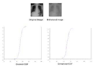
For this activity, I used an x-ray image whose histogram is not that spread along the grayscale range of values (0-255). Taking the PDF of the histogram, the plot has so may bump and curves.
By back projecting the original array of image to the CDF of its histogram, it enhances both the image and the histogram of the original image.
Below are the histograms , CDF , output image of the original image and the enhanced image:
The source code of this image enhancement is written below:
a = imread("G:\Documents and Settings\Semicon_2\Desktop\X-Ray.jpg");
n = size(a);
row = n(1);
col = n(2);
b = im2gray(a);
c = 255*b;
x = [0:255];
//Loop for Histogram//
for d = 1:256
counter = 0.0; //Initialize count
for i = 1:row // Number of rows
for j = 1:col // Number of columns
if c(i,j) == d
counter = counter + 1.0;
end
x(d) = counter;
end
end
end
x1 = x/max(x);
x2 = cumsum(x1);
x3 = x2/max(x2);
c2 = c;
//Loop for Back - Projection//
for i = 1:row// Number of rows
for j = 1:col// Number of columns
c2(i,j) = x3(c(i,j)+1) ;
end
end
c3 = floor(255*c2);
x4 = [0:255];
//Loop for the final histogram//
for d = 1:256
counter = 0.0; //Initialize count
for i = 1:row // Number of rows
for j = 1:col // Number of columns
if c3(i,j) == d
counter = counter + 1.0;
end
x4(d) = counter;
end
end
end
x5 = x4/max(x4);
x6 = cumsum(x5);
x7 = x6/max(x6);
scf(1)
plot(x7);
scf(2)
imshow(c2);
scf(3);scf(1)
plot(x7);
scf(2)
imshow(c2);
scf(3);
imshow(b);
My modified program which includes a desired function G(z) which is a hyperbolic tangent with a form:
G = tanh(16*(z-128)/255);
The process of back-projection shown in a figure below:The value of the new image will come from the desired CDF. The resulting image is shown below:
I acknowledge the help extended byElizabeth Prieto and Rafael Jaculbia in debugging my program. I give myself a grade of 9 for the reason that I found it hard to understand how back-projection part.
Source:
profile.myspace.com
Monday, June 30, 2008
Wednesday, June 25, 2008
Image types and basic image enhancement
Using the command imfinfo on scilab, properties of different image types were displayed here in my blog.
For Binary image:
Filesize: 19338 bytes
File format: JPEG
Width: 430
Height: 323
Depth: 8
Storage type: truecolor
Number Of Colors: 0
Resolution Unit: centimeter
X Resolution: 0
Y Resolution: 0
For Grayscale image:
Filesize: 19993 bytes
File format: JPEG
Width: 430
Height: 323
Depth: 8
Storage type: truecolor
Number Of Colors: 0
Resolution Unit: centimeter
X Resolution: 0
Y Resolution: 0
For Indexed image:
Filesize: 23422 bytes
File format: GIF
Width: 430
Height: 323
Depth: 8
Storage type: indexed
Number Of Colors: 256
Resolution Unit: centimeter
X Resolution: 0
Y Resolution: 0
For Truecolor image:
Filesize: 20414 bytes
File format: JPG
Width: 430
Height: 323
Depth: 8
Storage type: truecolor
Number Of Colors: 0
Resolution Unit: centimeter
X Resolution: 0
Y Resolution: 0
The information of my scanned image are listed below:
Filesize: 11225 bytes
File format: JPG
Width: 355
Height: 336
Depth: 8
Storage type: indexed
Number Of Colors: 256
Resolution Unit: inch
X Resolution: 0
Y Resolution: 0
The total number of pixel (area) of my image using pixel counting is 16423 pixels.
Using the software ImageJ, I can show the histogram of the grayscale of the scanned image. The ROI has a separation with the background.
I simulated the histogram of the image using Scilab. Below is the resulting histogram of the ImageJ and my simulation.
The first plot is the histogram from ImageJ. The second one is the histogram from simulations.
I posted my source code in getting both for the histogram and the area of the image. I inculded the simulation for thresholding...
a = imread("F:\AP 186\image\others\horge.jpg");
b = im2gray(a);
c = 255*b;
x = [0:255];
n = size(a);
row = n(1);
col = n(2);
for d = 1:256
counter = 0.0; //Initialize count
for i = 1:row // Number of rows
for j = 1:col // Number of columns
if c(i,j) == d
counter = counter + 1.0;
x(d) = counter;
end
end
end
end
//x will be the function for the histogram
//Thresholding
for i = 1:row // Number of rows
for j = 1:col // Number of columns
if c(i,j) < 240 //Choose best threshold from the histogram of the image
c(i,j) = 0;
end
end
end
d = 0.00390625*c;//To convert the value range from 0 to 1
//Getting the Area//
f = im2bw(d,0.01)
counter = 0.0; //Initialize count
for i = 1:row // Number of rows
for j = 1:col // Number of columns
if f(i,j) == 0
counter = counter + 1.0;
end
end
end
f1 = abs(f-1); //area
In this activity, Eduardo David helped me in debugging my program.
The grade that I will give myself is 10 because all of the programming was done by myself.
SOURCE:
www.freshpeel.com
Wednesday, June 18, 2008
Measurement of the Area for Different images
I made four different shapes:
1. Square
2. Circle
3. Triangle
4. Irregular shape
Using scilab, I made a program to get the area for each of the shapes I made. I posted the source code below:
a = imread("C:\Documents and Settings\AP186user15\Desktop\ryt.bmp");//command line for opening image file
b= im2bw(a,1);
[x,y] = follow(b);
c = size(x);
d = size(y);
c1 = c(1);
d1 = d(1);
x_1 = x;
y_1 = y;
x_1(2:c1) = x(1:c1-1);
x_1(1) = x(d1);
y_1(2:d1) = y(1:d1-1);
y_1(1) = y(d1);
initial = x.*y_1 - y.*x_1;
area = (0.5*(sum(initial)));
absolute_area = (area^2)^0.5;
//Getting the percent error //
Error = ((sum(b)-absolute_area)/sum(b))*100;
The resulting areas and the actual area:
Area | Pixel Count Area | Percent Error | |
Square | 88209 | 88804 | 0.67 |
Circle | 71552 | 71981 | 0.6 |
Triangle | 44999.5 | 45450 | 0.99 |
Irregular Shape | 48780 | 49383 | 1.22 |
For this program, Ed helped me in identifying errors in my program and Raf helped me understand the equation I used in obtaining the area of the image.
For this activity, I will give myself a grade of 9.5 / 10. It's not 10 because others helped me do this program.
Wednesday, June 11, 2008
The ratio of physical values on x -axis is 0.0005 per pixel
The ratio of physical values on y -axis is 0.0002 per pixel
The pixel location of the origin of the plot is at 30 pixels from the right and 211 below the origin of 314x235 pix picture.
The formulas used to relate the pixel location to the physical variables:
For x-axis;
[(X axis of the pixel location value)-30]*0.0005
For y-axis;
[211-(Y axis of the pixel location value)]*0.0002
Below are the values I tabulated
The superimposed plot of the scanned hand-written plot and the reconstructed plot
I will grade myself in this activity as 10.
The ratio of physical values on y -axis is 0.0002 per pixel
The pixel location of the origin of the plot is at 30 pixels from the right and 211 below the origin of 314x235 pix picture.
The formulas used to relate the pixel location to the physical variables:
For x-axis;
[(X axis of the pixel location value)-30]*0.0005
For y-axis;
[211-(Y axis of the pixel location value)]*0.0002
Below are the values I tabulated
X axis of the pixel location | Y axis of the pixel location | x | y |
50 | 149 | 10 | 12.4 |
70 | 106 | 20 | 21 |
110 | 76 | 40 | 27 |
150 | 74 | 60 | 27.4 |
190 | 83 | 80 | 25.6 |
230 | 99 | 100 | 22.4 |
The superimposed plot of the scanned hand-written plot and the reconstructed plot
I will grade myself in this activity as 10.
Subscribe to:
Posts (Atom)